Chapter 3 Data Wrangling

So far in our journey, we’ve seen how to look at data saved in data frames (Chapter 1) and how to create data visualizations using the grammar of graphics, which maps variables in a data frame to the aesthetic attributes of geometric objects (Chapter 2).

Recall that for some of our visualizations, we first needed to transform/modify existing data frames a little. For example, to create the linegraph in Figure 2.7 with measurements only for Chick 1, we first needed to pare down the ChickWeight data frame to a chick1_weight data frame consisting of only Chick == 1 rows. Thus, chick1_weight will have fewer rows than ChickWeight. We did this using the filter() function:

chick1_weight <- filter(ChickWeight, Chick == 1)

In this chapter, we’ll extend this example and we’ll introduce a series of functions from the dplyr package for data wrangling that will allow you to take a data frame and “wrangle” it (transform it) to suit your needs. Such functions include:

1. filter() and slice a data frame’s existing rows to only pick out a subset of rows.
2. select() a data frame’s existing columns to only keep a subset or rename existing columns.
3. summarize() one or more of a data frame’s columns/variables with a summary statistic. Examples of summary statistics include the median and interquartile range of chick weights as we saw in Section 2.7 on boxplots.
4. group_by() the rows of a data frame. In other words, assign different rows to be part of the same group. We can then combine group_by() with summarize() to report summary statistics for each group separately. For example, say you don’t want a single overall average weight on Day 21 for the chick_weight_d21 dataset, but rather four separate averages, one computed for each of the four Diet groups.
5. mutate() a data frame’s existing columns/variables to create new ones. For example, convert weight recordings from grams to ounces.
6. arrange() a data frame’s rows in a new order. For example, sort the rows of mammals in ascending or descending order of life_span.

Notice how we used computer_code font to describe the actions we want to take on our data frames. This is because the dplyr package for data wrangling has intuitively verb-named functions that are easy to remember.

There is a further benefit to learning to use the dplyr package for data wrangling: its similarity to the database querying language SQL (pronounced “sequel” or spelled out as “S”, “Q”, “L”). SQL (which stands for “Structured Query Language”) is used to manage large databases quickly and efficiently and is widely used by many institutions with a lot of data. While SQL is a topic left for a book or a course on database management, keep in mind that once you learn dplyr, you can learn SQL easily.

Chapter Learning Objectives

At the end of this chapter, you should be able to…
• Use pipes to make it easier to create and read complex code.
• Use data wrangling functions to rearrange a data frame, retrieve a subset of rows or columns, and create new variables.
• Calculate summary statistics, such as mean and median, for separate groups.

Needed packages

Let’s load all the packages needed for this chapter (this assumes you’ve already installed them). If needed, read Section 1.3 for information on how to install and load R packages.

library(dplyr)
library(ggplot2)
library(openintro)

3.1 The pipe operator: %>%

Before we start data wrangling, let’s first introduce a nifty tool that gets loaded with the dplyr package: the pipe operator %>% (also indicated as |>). The pipe operator allows us to combine multiple operations in R into a single sequential chain of actions.

Let’s start with a hypothetical example. Say you would like to perform a hypothetical sequence of operations on a hypothetical data frame x using hypothetical functions f(), g(), and h():

1. Take x then
2. Use x as an input to a function f() then
3. Use the output of f(x) as an input to a function g() then
4. Use the output of g(f(x)) as an input to a function h()

One way to achieve this sequence of operations is by using nesting parentheses as follows:

h(g(f(x)))

This code isn’t so hard to read since we are applying only three functions: f(), then g(), then h() and each of the functions is short in its name. Further, each of these functions also only has one argument. However, you can imagine that this will get progressively harder to read as the number of functions applied in your sequence increases and the arguments in each function increase as well. This is where the pipe operator %>% comes in handy. %>% takes the output of one function and then “pipes” it to be the input of the next function. Furthermore, a helpful trick is to read %>% as “then” or “and then.” For example, you can obtain the same output as the hypothetical sequence of functions as follows:

x %>% 
  f() %>% 
  g() %>% 
  h()

You would read this sequence as:

1. Take x then
2. Use this output as the input to the next function f() then
3. Use this output as the input to the next function g() then
4. Use this output as the input to the next function h()

So while both approaches achieve the same goal, the latter is much more human-readable because you can clearly read the sequence of operations line-by-line. But what are the hypothetical x, f(), g(), and h()? Throughout this chapter on data wrangling:

1. The starting value x will be a data frame. For example, the mammals data frame we explored in Section 1.4.2.
2. The sequence of functions, here f(), g(), and h(), will mostly be a sequence of any number of the data wrangling, verb-named functions we listed in the introduction to this chapter. For example, the filter(Chick == 1) function and argument we previewed earlier.
3. The result will be the transformed/modified data frame that you want. In our example, we’ll save the result in a new data frame by using the <- assignment operator with the name chick1_weight via chick1_weight <-.

chick1_weight <- ChickWeight %>% 
  filter(Chick == 1)

Much like when adding layers to a ggplot() using the + sign, you form a single chain of data wrangling operations by combining verb-named functions into a single sequence using the pipe operator %>%. Furthermore, much like how the + sign has to come at the end of lines when constructing plots, the pipe operator %>% has to come at the end of lines as well.

Keep in mind, there are many more advanced data wrangling functions than just those listed in the introduction to this chapter. However, just with these verb-named functions you’ll be able to perform a broad array of data wrangling tasks for the rest of this book.

3.2 filter rows

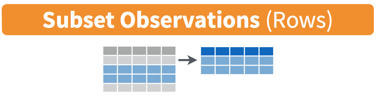
FIGURE 3.1: Diagram of filter() rows operation.

The filter() function here works much like the “Filter” option in Microsoft Excel; it allows you to specify criteria about the values of a variable in your dataset and then filters out only the rows that match that criteria.

We begin by focusing only on mammalian species in predationcategory 1. Run the following and look at the results in RStudio’s spreadsheet viewer to ensure that only species in predationcategory 1 are chosen

predation1 <- mammals %>% 
  filter(predation == 1)
View(predation1)

Note the order of the code. First, take the mammals data frame; then filter() the data frame so that only those where predation equals 1 are included. We test for equality using the double equal sign == and not a single equal sign =. In other words filter(predation = 1) will yield an error. This is a convention across many programming languages. If you are new to coding, you’ll probably forget to use the double equal sign == a few times before you get the hang of it.

You can use other operators beyond just the == operator that tests for equality:

• > corresponds to “greater than”
• < corresponds to “less than”
• >= corresponds to “greater than or equal to”
• <= corresponds to “less than or equal to”
• != corresponds to “not equal to.” The ! is used in many programming languages to indicate “not.”

Furthermore, you can combine multiple criteria using operators that make comparisons:

• | corresponds to “or”
• & corresponds to “and”

To see many of these in action, let’s filter mammals for mammalian species that are in predation category 1 or 2 and not in exposure category 1. Note that this example uses the ! “not” operator to pick rows that don’t match a criteria. As mentioned earlier, the ! can be read as “not.” Run the following:

predation_notexp1 <- mammals %>% 
  filter((predation == 1 | predation == 2) & exposure != 1)
predation_notexp1

# A tibble: 12 × 14
   species          body_wt brain_wt non_dreaming dreaming total_sleep life_span
   <fct>              <dbl>    <dbl>        <dbl>    <dbl>       <dbl>     <dbl>
 1 Cat                3.3       25.6         10.9      3.6        14.5      28  
 2 Echidna            3         25            8.6      0           8.6      50  
 3 Europeanhedgehog   0.785      3.5          6.6      4.1        10.7       6  
 4 Galago             0.2        5            9.5      1.2        10.7      10.4
 5 Genet              1.41      17.5          4.8      1.3         6.1      34  
 6 Gorilla          207        406           NA       NA          12        39.3
 7 Grayseal          85        325            4.7      1.5         6.2      41  
 8 Owlmonkey          0.48      15.5         15.2      1.8        17        12  
 9 Raccoon            4.288     39.2         NA       NA          12.5      13.7
10 Rhesusmonkey       6.8      179            8.4      1.2         9.6      29  
11 Rockhyrax(Heter…   0.75      12.3          5.7      0.9         6.6       7  
12 Slowloris          1.4       12.5         NA       NA          11        12.7
# ℹ 7 more variables: gestation <dbl>, predation <int>, exposure <int>,
#   danger <int>, wt_in_lb <dbl>, wt_in_oz <dbl>, oz_per_year <dbl>

As expected, the predation_notexp1 data frame contains a subset, 12 rows, of the 62 rows in the original mammals data frame.

This alternative code where we do not select species that are exposure category 1 achieves the same aim:

predation_notexp1 <- mammals %>% 
  filter((predation == 1 | predation == 2) & !exposure == 1)
predation_notexp1

Note that even though colloquially speaking one might say “all mammalian species that are predation category 1 and 2,” in terms of computer operations, we really mean “all mammalian species that are predation category 1 or 2.” For a given row in the data, predation can be 1, or 2, or something else, but not both 1 and 2 at the same time.

We can often skip the use of & and just separate our conditions with a comma. The following code will return the identical output predation_notexp1 as the previous code:

predation_notexp1 <- mammals %>% 
  filter((predation == 1 | predation == 2), !exposure == 1)
predation_notexp1

Now say we have a larger number of categories we want to filter for, say a subset of species such as "Africanelephant", "Asianelephant", "Deserthedgehog", and "Europeanhedgehog". We could continue to use the | (or) operator:

many_species <- mammals %>% 
  filter(species == "Africanelephant" | species == "Asianelephant" | species == "Deserthedgehog" | species == "Europeanhedgehog")

but as we progressively include more categories, this will get unwieldy to write. A slightly shorter approach uses the %in% operator along with the c() function. Recall from Subsection 1.2.1 that the c() function “combines” or “concatenates” values into a single vector of values.

many_species <- mammals %>% 
  filter(species %in% c("Africanelephant", "Asianelephant", "Deserthedgehog", "Europeanhedgehog"))
many_species

# A tibble: 4 × 14
  species           body_wt brain_wt non_dreaming dreaming total_sleep life_span
  <fct>               <dbl>    <dbl>        <dbl>    <dbl>       <dbl>     <dbl>
1 Africanelephant  6654       5712           NA       NA           3.3      38.6
2 Asianelephant    2547       4603            2.1      1.8         3.9      69  
3 Deserthedgehog      0.55       2.4          7.6      2.7        10.3      NA  
4 Europeanhedgehog    0.785      3.5          6.6      4.1        10.7       6  
# ℹ 7 more variables: gestation <dbl>, predation <int>, exposure <int>,
#   danger <int>, wt_in_lb <dbl>, wt_in_oz <dbl>, oz_per_year <dbl>

This code filters mammals for all mammalian species where species is in the vector of species c("Africanelephant", "Asianelephant", "Deserthedgehog", "Europeanhedgehog"). Both outputs of many_species are the same, but as you can see the latter takes much less energy to code. The %in% operator is useful for looking for matches commonly in one vector/variable compared to another.

As a final note, we recommend that filter() should be among the first verbs you consider applying to your data. This cleans your dataset to only those rows you care about, or put differently, it narrows down the scope of your data frame to just the observations you care about.

Learning check

(LC3.1) Adapt the previous code using the “not” operator ! to filter only the species that are not danger category 4 or 5 in the mammals data frame.

3.3 slice rows

Similar to filter, the slice function function returns a subset of rows from a data frame. While filter returns the rows that match a specified criteria about the values of a variable (e.g., species == "Cat"), the slice function returns rows based on their positions. For example, let’s slice the first 5 rows of the mammals data frame:

mammals %>% slice(1:5)

However, even more useful is a derivative of slice called slice_max that allow us to retrieve rows with the top values of a specified variable. For example, we can return a data frame of the 5 mammalian species with the longest life spans. Observe that we set the number of values to return to n = 5 and order_by = life_span to indicate that we want the rows corresponding to the top 5 values of life_span.

mammals %>% slice_max(n = 5, order_by = life_span)

See the help file for slice() by running ?slice for more information about its related functions.

Learning check

(LC3.2) Repeat the previous command substituting the function slice_head for slice_max. How does the output differ?

(LC3.3) Create a new data frame notLongLife that shows the rows of the mammals data frame with the 5 smallest values of the life_span variable. (Check the slice() help file for hints.)

3.4 select variables

We recommended that you consider applying the filter() function to your data to narrow down the scope of your data frame to just the observations you care about. It may also be the case that you are only interested in a subset of the variables in your dataset. For example, the mammals data frame has 14 variables, but typically only a few variables will be of interest for a particular analysis. You can identify the names of these 14 variables by running the glimpse() function from the dplyr package:

glimpse(mammals)

In the same way that filter and slice return a subset of rows, the select function and its selection helpers allow us to return a subset of columns from a data frame as illustrated in Figure 3.2.

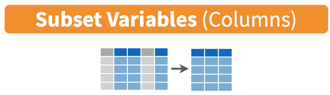
FIGURE 3.2: Diagram of select() columns.

Returning to many_species, our data frame with four mammalian species, we might only really be interested in the variables species, body_wt and danger. However, with the current data frame, it’s a bit difficult to compare these columns among all the others:

many_species

# A tibble: 4 × 14
  species           body_wt brain_wt non_dreaming dreaming total_sleep life_span
  <fct>               <dbl>    <dbl>        <dbl>    <dbl>       <dbl>     <dbl>
1 Africanelephant  6654       5712           NA       NA           3.3      38.6
2 Asianelephant    2547       4603            2.1      1.8         3.9      69  
3 Deserthedgehog      0.55       2.4          7.6      2.7        10.3      NA  
4 Europeanhedgehog    0.785      3.5          6.6      4.1        10.7       6  
# ℹ 7 more variables: gestation <dbl>, predation <int>, exposure <int>,
#   danger <int>, wt_in_lb <dbl>, wt_in_oz <dbl>, oz_per_year <dbl>

Examining these columns is much easier if we work with a smaller data frame by select()ing the desired variables:

slim_many_species <- many_species %>% 
  select(species, body_wt, danger)

This slimmer data frame makes it easy to verify that we correctly filtered for species and also helps us to see the various ways that body weight relates to the danger faced by each species from other animals:

slim_many_species

# A tibble: 4 × 3
  species           body_wt danger
  <fct>               <dbl>  <int>
1 Africanelephant  6654          3
2 Asianelephant    2547          4
3 Deserthedgehog      0.55       2
4 Europeanhedgehog    0.785      2

Let’s say instead you want to drop, or de-select, certain variables. For example, perhaps you want to drop the gestation variable. We can deselect gestation by using the - sign:

mammals_10cols <- mammals %>% select(-gestation)

Another way of selecting columns/variables is by specifying a range of columns. For example, we might want to only focus on the sleep-related variables for the mammalian species:

mammals_sleep <- mammals %>% select(species, non_dreaming:total_sleep)
mammals_sleep

# A tibble: 62 × 4
   species                non_dreaming dreaming total_sleep
   <fct>                         <dbl>    <dbl>       <dbl>
 1 Africanelephant                NA       NA           3.3
 2 Africangiantpouchedrat          6.3      2           8.3
 3 ArcticFox                      NA       NA          12.5
 4 Arcticgroundsquirrel           NA       NA          16.5
 5 Asianelephant                   2.1      1.8         3.9
 6 Baboon                          9.1      0.7         9.8
 7 Bigbrownbat                    15.8      3.9        19.7
 8 Braziliantapir                  5.2      1           6.2
 9 Cat                            10.9      3.6        14.5
10 Chimpanzee                      8.3      1.4         9.7
# ℹ 52 more rows

The select() function can also be used to reorder columns when combined with the everything() helper function. For example, suppose we want the species and sleep-related variables to appear first, while not discarding the rest of the variables. In the following code, everything() will pick up all remaining variables:

mammals_reorder <- mammals %>% select(species, non_dreaming:total_sleep, everything())
glimpse(mammals_reorder)

See the help file for select() by running ?select for more information about other selection helpers.

Learning check

(LC3.4) Run the code mammals %>% select(ends_with("wt")) to select columns with names that end with “wt”. How many columns are returned?

(LC3.5) Use the contains() helper function to select columns from the mammals data frame that contain “dream”. How many columns are returned?

(LC3.6) What if you forgot to include the double-quotes for the first command above? Run the code mammals %>% select(ends_with(wt)) to see what happens.

The last command shows an example of what happens when you forget to include double-quotes. If you see an Error message about an object ... not found, try adding double-quotes to see if that fixes the problem.

3.4.1 rename variables

Another useful function similar to select() is rename(), which as you may have guessed changes the name of specified variables. Suppose we want to rename the danger variable to something more understandable, such as danger_faced:

mammals %>% 
  rename(danger_faced = danger)

Only the name of the specified variable has changed, and all of the other variables remain intact and unchanged. Note that here we used a single = sign within the rename(). For example, danger_faced = danger renames the danger variable to have the new name danger_faced. This is because we are not testing for equality like we would using ==. Instead we want to assign a new variable danger_faced to have the same values as danger and then delete the variable danger.

Tip: New dplyr users often forget that the new variable name comes before the equal sign, followed by the old variable. You can remember this as “New Before Old”. Tip 2: Avoid spaces and special symbols in your variable names, which in our experience can cause problems in R.

Pro-tip: We can also rename variables as we select() them from a data frame:

mammals %>% 
  select(species, danger_faced = danger)

# A tibble: 62 × 2
   species                danger_faced
   <fct>                         <int>
 1 Africanelephant                   3
 2 Africangiantpouchedrat            3
 3 ArcticFox                         1
 4 Arcticgroundsquirrel              3
 5 Asianelephant                     4
 6 Baboon                            4
 7 Bigbrownbat                       1
 8 Braziliantapir                    4
 9 Cat                               1
10 Chimpanzee                        1
# ℹ 52 more rows

Here we selected two columns from mammals, changing the name of the second one in the process.

3.5 summarize variables

Another common task when working with data frames is to compute summary statistics. Summary statistics are single numerical values that summarize a large number of values. Commonly known examples of summary statistics include the mean (also called the average) and the median (the middle value). Other examples of summary statistics that might not immediately come to mind include the sum, the smallest value also called the minimum, the largest value also called the maximum, and the standard deviation, a measure of the variability or “spread” in the values. See Appendix A.1 for a glossary of such summary statistics.

Let’s calculate two summary statistics of the life_span variable in the mammals data frame: the mean and standard deviation. To compute these summary statistics, we need the mean() and sd() summary functions in R. Summary functions in R take in many values and return a single value, as illustrated in Figure 3.3.

FIGURE 3.3: Diagram illustrating a summary function in R.

More precisely, we’ll use the mean() and sd() summary functions within the summarize() function from the dplyr package. Note you can also use the British English spelling of summarise(). As shown in Figure 3.4, the summarize() function takes in a data frame and returns a data frame with only one row corresponding to the summary statistics.

FIGURE 3.4: Diagram of summarize() rows.

We’ll save the results in a new data frame called summary_mammals that will have two columns/variables: the mean and the std_dev:

summary_mammals <- mammals %>% 
  summarize(mean = mean(life_span), std_dev = sd(life_span))
summary_mammals

# A tibble: 1 × 2
   mean std_dev
  <dbl>   <dbl>
1    NA      NA

Why are the values returned NA? As we saw in Subsection 2.3.1, NA is how R encodes missing values . By default any time you try to calculate a summary statistic of a variable that has one or more NA missing values in R, NA is returned. To work around this fact, you can set the na.rm argument of each summary function to TRUE, where rm is short for “remove”; this will ignore any NA missing values and only return the summary value for all non-missing values.

The code that follows computes the mean and standard deviation of all non-missing values of life_span:

summary_mammals <- mammals %>% 
  summarize(mean = mean(life_span, na.rm = TRUE), 
            std_dev = sd(life_span, na.rm = TRUE))
summary_mammals

# A tibble: 1 × 2
     mean std_dev
    <dbl>   <dbl>
1 19.8776 18.2063

Notice how the na.rm = TRUE are used as arguments to the mean() and sd() summary functions individually, and not to the summarize() function.

However, one needs to be cautious whenever ignoring missing values. In the upcoming Learning checks questions, we’ll consider the possible ramifications of blindly sweeping rows with missing values “under the rug.” This is in fact why the na.rm argument to any summary statistic function in R is set to FALSE by default. In other words, R does not ignore rows with missing values by default. R is alerting you to the presence of missing data and you should be mindful of this absence and any potential causes of this absence throughout your analysis.

What are other summary functions we can use inside the summarize() verb to compute summary statistics? As seen in the diagram in Figure 3.3, you can use any summary function in R that takes many values and returns just one. Here are just a few:

• mean(): the average
• sd(): the standard deviation, which is a measure of spread
• min() and max(): the minimum and maximum values, respectively
• IQR(): interquartile range
• sum(): the total amount when adding multiple numbers
• n(): a count of the number of rows in each group. This particular summary function will make more sense when group_by() is covered in Section 3.6.

In Section 3.7, we will introduce the skim() function, which can save you a lot of time writing code to calculate the most common summary statistics.

Learning check

(LC3.7) A doctor is studying the effect of smoking on lung cancer for a large number of patients who have records measured at five-year intervals. She notices that a large number of patients have missing data points because the patient has died, so she chooses to ignore these patients in her analysis. What is wrong with this doctor’s approach?

(LC3.8) Modify the earlier summarize() function code that creates the summary_mammals data frame to also use the n() summary function: summarize(... , count = n()). What does the returned value correspond to?

(LC3.9) Why doesn’t the following code work? Run the code line-by-line instead of all at once, and then look at the data. In other words, run summary2_mammals <- mammals %>% summarize(mean = mean(life_span, na.rm = TRUE)) first.

summary2_mammals <- mammals %>%   
  summarize(mean = mean(life_span, na.rm = TRUE)) %>% 
  summarize(std_dev = sd(life_span, na.rm = TRUE))

3.6 group_by rows

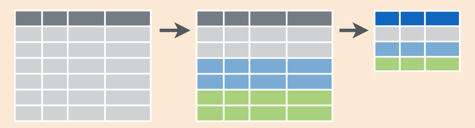
FIGURE 3.5: Diagram of group_by() and summarize().

Above we calculated the mean life_span of mammals. Say instead of a single mean life_span for a dataset, we would like to compute the mean life_spans of species in different predation categories separately, that is, the mean life_span split by predation. We can do this by “grouping” the life_span observations by the values of another variable, in this case by the values of the variable predation. Run the following code:

summary_pred_life <- mammals %>% 
  group_by(predation) %>% 
  summarize(mean = mean(life_span, na.rm = TRUE), 
            std_dev = sd(life_span, na.rm = TRUE))
summary_pred_life

# A tibble: 5 × 3
  predation    mean std_dev
      <int>   <dbl>   <dbl>
1         1 29.1571 24.5232
2         2 13.2923 12.8962
3         3 15.3909 20.6090
4         4 19.1143 11.7115
5         5 20.6769 12.9310

This code is similar to the code that created summary_mammals, but with an extra group_by() command added before the summarize(). Grouping the mammals dataset by predation and then applying the summarize() functions yields a data frame that displays the mean and standard deviation length split by the different predation categories.

It is important to note that the group_by() function doesn’t change data frames by itself. Rather it changes the meta-data, or data about the data, specifically the grouping structure. It is only after we apply the summarize() function that the data frame changes.

For example, let’s consider the mammals data frame again. Run this code:

mammals

# A tibble: 62 × 14
   species          body_wt brain_wt non_dreaming dreaming total_sleep life_span
   <fct>              <dbl>    <dbl>        <dbl>    <dbl>       <dbl>     <dbl>
 1 Africanelephant 6654       5712           NA       NA           3.3      38.6
 2 Africangiantpo…    1          6.6          6.3      2           8.3       4.5
 3 ArcticFox          3.385     44.5         NA       NA          12.5      14  
 4 Arcticgroundsq…    0.92       5.7         NA       NA          16.5      NA  
 5 Asianelephant   2547       4603            2.1      1.8         3.9      69  
 6 Baboon            10.55     179.5          9.1      0.7         9.8      27  
 7 Bigbrownbat        0.023      0.3         15.8      3.9        19.7      19  
 8 Braziliantapir   160        169            5.2      1           6.2      30.4
 9 Cat                3.3       25.6         10.9      3.6        14.5      28  
10 Chimpanzee        52.16     440            8.3      1.4         9.7      50  
# ℹ 52 more rows
# ℹ 7 more variables: gestation <dbl>, predation <int>, exposure <int>,
#   danger <int>, wt_in_lb <dbl>, wt_in_oz <dbl>, oz_per_year <dbl>

Observe that the first line of the output reads # A tibble: 62 x 14. This is an example of meta-data, in this case the number of observations/rows and variables/columns in mammals. The actual data itself are the subsequent table of values. Now let’s pipe the mammals data frame into group_by(predation):

mammals %>% 
  group_by(predation)

# A tibble: 62 × 14
# Groups:   predation [5]
   species          body_wt brain_wt non_dreaming dreaming total_sleep life_span
   <fct>              <dbl>    <dbl>        <dbl>    <dbl>       <dbl>     <dbl>
 1 Africanelephant 6654       5712           NA       NA           3.3      38.6
 2 Africangiantpo…    1          6.6          6.3      2           8.3       4.5
 3 ArcticFox          3.385     44.5         NA       NA          12.5      14  
 4 Arcticgroundsq…    0.92       5.7         NA       NA          16.5      NA  
 5 Asianelephant   2547       4603            2.1      1.8         3.9      69  
 6 Baboon            10.55     179.5          9.1      0.7         9.8      27  
 7 Bigbrownbat        0.023      0.3         15.8      3.9        19.7      19  
 8 Braziliantapir   160        169            5.2      1           6.2      30.4
 9 Cat                3.3       25.6         10.9      3.6        14.5      28  
10 Chimpanzee        52.16     440            8.3      1.4         9.7      50  
# ℹ 52 more rows
# ℹ 7 more variables: gestation <dbl>, predation <int>, exposure <int>,
#   danger <int>, wt_in_lb <dbl>, wt_in_oz <dbl>, oz_per_year <dbl>

Observe that now there is additional meta-data: # Groups: predation [5] indicating that the grouping structure meta-data has been set based on the 5 possible levels of the categorical variable predation. On the other hand, observe that the data has not changed: it is still a table of 62 \(\times\) 14 values.

Only by combining a group_by() with another data wrangling operation, in this case summarize(), will the data actually be transformed.

mammals %>% 
  group_by(predation) %>% 
  summarize(avg_life = mean(life_span, na.rm = TRUE))

# A tibble: 5 × 2
  predation avg_life
      <int>    <dbl>
1         1  29.1571
2         2  13.2923
3         3  15.3909
4         4  19.1143
5         5  20.6769

If you would like to remove this grouping structure meta-data, we can pipe the resulting data frame into the ungroup() function:

mammals %>% 
  group_by(predation) %>% 
  ungroup()

# A tibble: 62 × 14
   species          body_wt brain_wt non_dreaming dreaming total_sleep life_span
   <fct>              <dbl>    <dbl>        <dbl>    <dbl>       <dbl>     <dbl>
 1 Africanelephant 6654       5712           NA       NA           3.3      38.6
 2 Africangiantpo…    1          6.6          6.3      2           8.3       4.5
 3 ArcticFox          3.385     44.5         NA       NA          12.5      14  
 4 Arcticgroundsq…    0.92       5.7         NA       NA          16.5      NA  
 5 Asianelephant   2547       4603            2.1      1.8         3.9      69  
 6 Baboon            10.55     179.5          9.1      0.7         9.8      27  
 7 Bigbrownbat        0.023      0.3         15.8      3.9        19.7      19  
 8 Braziliantapir   160        169            5.2      1           6.2      30.4
 9 Cat                3.3       25.6         10.9      3.6        14.5      28  
10 Chimpanzee        52.16     440            8.3      1.4         9.7      50  
# ℹ 52 more rows
# ℹ 7 more variables: gestation <dbl>, predation <int>, exposure <int>,
#   danger <int>, wt_in_lb <dbl>, wt_in_oz <dbl>, oz_per_year <dbl>

Observe how the # Groups: predation [5] meta-data is no longer present.

Let’s now revisit the n() counting summary function we briefly introduced previously. Recall that the n() function counts rows. This is opposed to the sum() summary function that returns the sum of a numerical variable. For example, suppose we’d like to count how many mammalian species were in each predation group:

by_pred <- mammals %>% 
  group_by(predation) %>% 
  summarize(count = n())
by_pred

# A tibble: 5 × 2
  predation count
      <int> <int>
1         1    14
2         2    15
3         3    12
4         4     7
5         5    14

We see that the greatest number of species are in predation category 2 and the fewest in category 4.

3.6.1 Grouping by more than one variable

You are not limited to grouping by one variable. Say you want to know the number of species of each predation category for each exposure level. We can also group by this second variable using group_by(predation, exposure):

by_pred_exp <- mammals %>% 
  group_by(predation, exposure) %>% 
  summarize(count = n())
by_pred_exp

# A tibble: 19 × 3
# Groups:   predation [5]
   predation exposure count
       <int>    <int> <int>
 1         1        1    10
 2         1        2     2
 3         1        3     1
 4         1        4     1
 5         2        1     7
 6         2        2     7
 7         2        3     1
 8         3        1     7
 9         3        2     2
10         3        5     3
11         4        1     2
12         4        3     1
13         4        4     3
14         4        5     1
15         5        1     1
16         5        2     2
17         5        3     1
18         5        4     1
19         5        5     9

Why do we group_by(predation, exposure) and not group_by(predation) and then group_by(exposure)? Let’s investigate:

by_pred_exp_incorrect <- mammals %>% 
  group_by(predation) %>% 
  group_by(exposure) %>% 
  summarize(count = n())
by_pred_exp_incorrect

# A tibble: 5 × 2
  exposure count
     <int> <int>
1        1    27
2        2    13
3        3     4
4        4     5
5        5    13

What happened here is that the second group_by(exposure) overwrote the grouping structure meta-data of the earlier group_by(predation), so that in the end we are only grouping by exposure. The lesson here is if you want to group_by() two or more variables, you should include all the variables at the same time in the same group_by() adding a comma between the variable names.

Learning check

(LC3.10) Examining the summary_pred_life data frame, in which predation category do mammalian species have the longest average life span? Which predation category shows the greatest variation in life spans?

(LC3.11) What code would be required to get the mean and standard deviation of life_span for each danger level of mammals?

(LC3.12) Recreate by_pred_exp, but instead of grouping via group_by(predation, exposure), group variables in the reverse order group_by(exposure, predation). What differs in the resulting dataset?

(LC3.13) How could we identify how many mammalian species are in each danger level?

(LC3.14) How does the filter() operation differ from a group_by() followed by a summarize()?

3.7 mutate existing variables

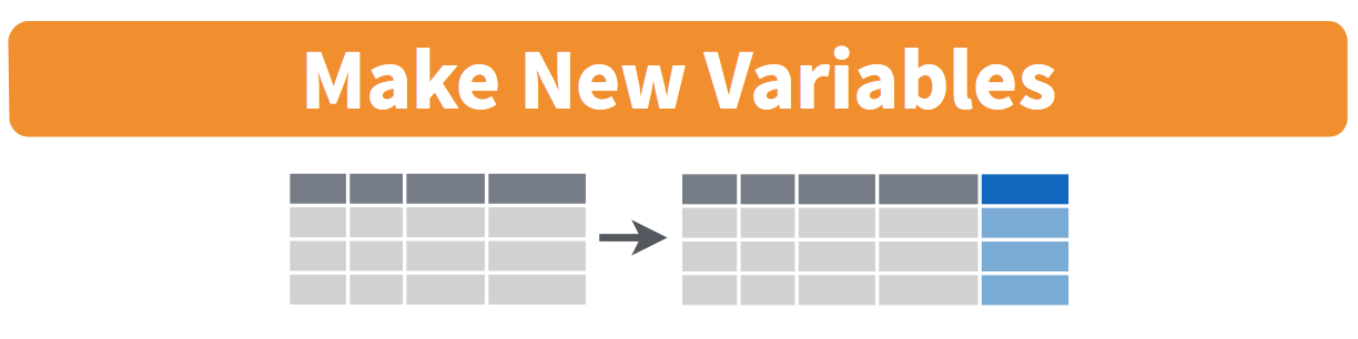
FIGURE 3.6: Diagram of mutate() columns.

Another common transformation of data is to create/compute new variables based on existing ones. For example, say you are more comfortable thinking of weight in pounds (lb) instead of kilograms (kg). The formula to convert weights from kg to lb is

\[ \text{weight in lb} = {\text{weight in kg}} \cdot {2.205} \]

We can apply this formula to the body_wt variable using the mutate() function from the dplyr package, which takes existing variables and mutates them to create new ones.

mammals <- mammals %>% 
  mutate(wt_in_lb = body_wt * 2.205)
mammals

# A tibble: 62 × 14
   species          body_wt brain_wt non_dreaming dreaming total_sleep life_span
   <fct>              <dbl>    <dbl>        <dbl>    <dbl>       <dbl>     <dbl>
 1 Africanelephant 6654       5712           NA       NA           3.3      38.6
 2 Africangiantpo…    1          6.6          6.3      2           8.3       4.5
 3 ArcticFox          3.385     44.5         NA       NA          12.5      14  
 4 Arcticgroundsq…    0.92       5.7         NA       NA          16.5      NA  
 5 Asianelephant   2547       4603            2.1      1.8         3.9      69  
 6 Baboon            10.55     179.5          9.1      0.7         9.8      27  
 7 Bigbrownbat        0.023      0.3         15.8      3.9        19.7      19  
 8 Braziliantapir   160        169            5.2      1           6.2      30.4
 9 Cat                3.3       25.6         10.9      3.6        14.5      28  
10 Chimpanzee        52.16     440            8.3      1.4         9.7      50  
# ℹ 52 more rows
# ℹ 7 more variables: gestation <dbl>, predation <int>, exposure <int>,
#   danger <int>, wt_in_lb <dbl>, wt_in_oz <dbl>, oz_per_year <dbl>

In this code, we mutate() the mammals data frame by creating a new variable wt_in_lb = body_wt * 2.205 and then overwrite the original mammals data frame. Why did we overwrite the data frame mammals, instead of assigning the result to a new data frame like mammals_new? As a rough rule of thumb, as long as you are not losing original information that you might need later, it’s acceptable practice to overwrite existing data frames with updated ones, as we did here. On the other hand, why did we not overwrite the variable body_wt, but instead created a new variable called wt_in_lb? Because if we did this, we would have erased the original information contained in body_wt of weights in grams that may still be valuable to us.

Let’s now compute average body weights of mammalian species in different predation categories in both kg and lb using the group_by() and summarize() code we saw in Section 3.6:

summary_pred_wt <- mammals %>% 
  group_by(predation) %>% 
  summarize(mean_wt_in_kg = mean(body_wt, na.rm = TRUE), 
            mean_wt_in_lb = mean(wt_in_lb, na.rm = TRUE))
summary_pred_wt

# A tibble: 5 × 3
  predation mean_wt_in_kg mean_wt_in_lb
      <int>         <dbl>         <dbl>
1         1       43.9234      96.8512 
2         2        1.973        4.35046
3         3      770.714     1699.42   
4         4       53.8301     118.695  
5         5      146.792      323.675  

Let’s look at some summary statistics of the wt_in_lb variable by considering multiple summary functions at once in the same summarize() code:

lb_summary <- mammals %>% 
  summarize(
    min = min(wt_in_lb, na.rm = TRUE),
    q1 = quantile(wt_in_lb, 0.25, na.rm = TRUE),
    median = quantile(wt_in_lb, 0.5, na.rm = TRUE),
    q3 = quantile(wt_in_lb, 0.75, na.rm = TRUE),
    max = max(wt_in_lb, na.rm = TRUE),
    mean = mean(wt_in_lb, na.rm = TRUE),
    sd = sd(wt_in_lb, na.rm = TRUE),
    missing = sum(is.na(wt_in_lb))
  )
lb_summary

# A tibble: 1 × 8
       min    q1  median      q3     max    mean      sd missing
     <dbl> <dbl>   <dbl>   <dbl>   <dbl>   <dbl>   <dbl>   <int>
1 0.011025 1.323 7.37021 106.287 14672.1 438.332 1982.64       0

We see for example that the mean weight for all mammalian species is about 438 pounds, while the heaviest species is 14,672 pounds!

However, typing out all these summary statistic functions in summarize() is long and tedious. Fortunately, there is a much more succinct way to compute a variety of common summary statistics using the skim() function from the skimr package. This function takes in a data frame, “skims” it, and returns commonly used summary statistics.

Let’s select the wt_in_lb column from mammals and pipe it into the skim() function:

mammals %>% select(wt_in_lb) %>% skim()

For the numerical variable wt_in_lb, skim() returns:

• n_missing: the number of missing values
• complete_rate: the proportion of complete values
• mean: the average
• sd: the standard deviation
• p0: the 0th percentile: the value at which 0% of observations are smaller than it (the minimum value)
• p25: the 25th percentile: the value at which 25% of observations are smaller than it (the 1st quartile)
• p50: the 50th percentile: the value at which 50% of observations are smaller than it (the 2nd quartile and more commonly called the median)
• p75: the 75th percentile: the value at which 75% of observations are smaller than it (the 3rd quartile)
• p100: the 100th percentile: the value at which 100% of observations are smaller than it (the maximum value)

Recall from Section 2.5 that since wt_in_lb is a numerical variable, we can visualize its distribution using a histogram.

ggplot(data = mammals, mapping = aes(x = wt_in_lb)) +
  geom_histogram(color = "white", boundary = 0, binwidth = 200)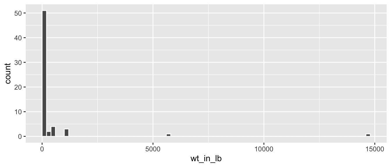

FIGURE 3.7: Histogram of wt_in_lb variable.

The resulting histogram in Figure 3.7 provides a different perspective on the wt_in_lb variable than the summary statistics we computed earlier. For example, note that most values of wt_in_lb are right around 0.

To close out our discussion on the mutate() function to create new variables, note that we can create multiple new variables at once in the same mutate() code. Furthermore, within the same mutate() code we can refer to new variables we just created, as shown in this example:

mammals <- mammals %>% 
  mutate(
    wt_in_oz = wt_in_lb * 16,
    oz_per_year = wt_in_oz / life_span
  )

Learning check

(LC3.15) What can we say about the distribution of wt_in_lb? Describe it in a few sentences using the plot and the lb_summary data frame values.

3.8 arrange and sort rows

One of the most commonly performed data wrangling tasks is to sort a data frame’s rows in the alphanumeric order of one of the variables. The dplyr package’s arrange() function allows us to sort/reorder a data frame’s rows according to the values of the specified variable.

Suppose we are interested in determining the predation level most common among mammalian species:

freq_pred <- mammals %>% 
  group_by(predation) %>% 
  summarize(num_species = n())
freq_pred

# A tibble: 5 × 2
  predation num_species
      <int>       <int>
1         1          14
2         2          15
3         3          12
4         4           7
5         5          14

Observe that by default the rows of the resulting freq_pred data frame are sorted in numerical order of predation category. Say instead we would like to see the same data, but sorted from the most to the least number of species (num_species) instead:

freq_pred %>% 
  arrange(num_species)

# A tibble: 5 × 2
  predation num_species
      <int>       <int>
1         4           7
2         3          12
3         1          14
4         5          14
5         2          15

This is, however, the opposite of what we want. The rows are sorted with the least frequently preferred habitats displayed first. This is because arrange() always returns rows sorted in ascending order by default. To switch the ordering to be in “descending” order instead, we use the desc() function as so:

freq_pred %>% 
  arrange(desc(num_species))

# A tibble: 5 × 2
  predation num_species
      <int>       <int>
1         2          15
2         1          14
3         5          14
4         3          12
5         4           7

3.9 Conclusion

3.9.1 Summary table

Let’s recap our data wrangling verbs in Table 3.1. Using these verbs and the pipe %>% operator from Section 3.1, you’ll be able to write easily legible code to perform almost all the data wrangling and data transformation necessary for the rest of this book.

TABLE 3.1: Summary of data wrangling verbs

Verb	Data wrangling operation
filter()	Pick out a subset of rows based on values of a variable
slice()	Pick out a subset of rows based on row number
select()	Pick out a subset of columns based on name or other criteria
summarize()	Summarize many values to one using a summary statistic function like mean(), median(), etc.
group_by()	Add grouping structure to rows in data frame. Note this does not change values in data frame, rather only the meta-data
mutate()	Create new variables by mutating existing ones
arrange()	Arrange rows of a data variable in ascending (default) or descending order

3.9.2 Additional resources

If you want to further unlock the power of the dplyr package for data wrangling, we suggest that you check out RStudio’s “Data Transformation with dplyr” cheatsheet. This cheatsheet summarizes much more than what we’ve discussed in this chapter, including more advanced data wrangling functions, while providing quick and easy-to-read visual descriptions. You can access this cheatsheet by going to the RStudio Menu Bar and selecting “Help -> Cheatsheets -> Data Transformation with dplyr.”

On top of the data wrangling verbs and examples we presented in this section, if you’d like to see more examples of using the dplyr package for data wrangling, check out Chapter 5 of R for Data Science (Grolemund and Wickham 2017).

3.9.3 What’s to come?

So far in this book, we’ve explored, visualized, and wrangled data saved in data frames. These data frames were saved in a spreadsheet-like format: in a rectangular shape with a certain number of rows corresponding to observations and a certain number of columns corresponding to variables describing these observations.

We’ll see in the upcoming Chapter 4 that there are actually two ways to represent data in spreadsheet-type rectangular format: (1) “wide” format and (2) “tall/narrow” format. The tall/narrow format is also known as “tidy” format in R user circles. While the distinction between “tidy” and non-“tidy” formatted data is subtle, it has immense implications for our data science work. This is because almost all the packages used in this book, including the ggplot2 package for data visualization and the dplyr package for data wrangling, assume that all data frames are in “tidy” format.

References

Grolemund, Garrett, and Hadley Wickham. 2017. R for Data Science. First. Sebastopol, CA: O’Reilly Media. https://r4ds.had.co.nz/.